Use YAML to style the plot function¶

This tutorial is aimed at beginners with no prior experience using YAML. You’ll learn by working through a small, hands-on example. Step by step, you’ll build a function called plot_yaml() that reads a YAML file and uses it to define the style options of MATLAB’s plot() function.

Setup¶

To follow this tutorial, you can use either a local installation of MATLAB (R2019b or newer) or MATLAB Online. Before you begin, create a new empty folder called yaml_tutorial/. You’ll use this folder to save files and work through the steps of the tutorial.

Install the YAML package in MATLAB¶

Download version v1.6.0 of the yaml package from the official GitHub repository:

https://github.com/MartinKoch123/yaml/archive/refs/tags/v1.6.0.zip

Move the downloaded ZIP file into yaml_tutorial/ and unzip it. You should now have a folder named yaml-1.6.0/.

Ensure the MATLAB Current Folder is set to yaml_tutorial/ and run the following command to add the package to MATLAB’s path:

>> addpath(genpath('yaml-1.6.0'));

Check that the package has been installed correctly by running the following command in the MATLAB command window:

>> help yaml

Contents of yaml namespace:

   Tests - yaml.Tests is a class.
    dump - Convert data to yaml string
dumpFile - Write data to yaml file.
    load - yaml.LOAD Parse yaml string
loadFile - Read yaml file.

If you see any different message, the package wasn’t added to MATLAB’s path correctly. Make sure the yaml-1.6.0/ folder and its subfolders are included.

Step 1: Create a YAML file for plot styles¶

Let’s create a YAML file called config.yaml to store the style options for the plot() function.

Define the following style options (LineStyle, LineWidth, and Color) in a MATLAB struct:

>> config.LineStyle = ':';
>> config.LineWidth = 2;
>> config.Color = [0.4, 0.2, 1.0];
>> config

config =

  struct with fields:

    LineStyle: ':'
    LineWidth: 2
        Color: [0.4000 0.2000 1]

Use the yaml.dumpFile() function to export this variable into a YAML file. This function automatically converts the MATLAB structure into the YAML format:

>> yaml.dumpFile('config.yaml', config);

Note that a new file config.yaml has been created. Open this file with the MATLAB editor and check that its content is the following:

config.yaml¶

LineStyle: ':'
LineWidth: 2.0
Color: [0.4, 0.2, 1.0]

The config.yaml file stores the same data as the MATLAB config variable, using YAML syntax. Although YAML looks similar to MATLAB, you don’t need to understand its syntax yet. For now, just observe how the information is automatically translated.

Step 2: Load YAML configuration into MATLAB¶

Let’s load the style options stored in the config.yaml YAML file back into a MATLAB variable.

Clear all workspace variables using the following command:

>> clear all;

Use the yaml.loadFile() function to load the data of config.yaml file:

>> config = yaml.loadFile('config.yaml', 'ConvertToArray', true)

config =

  struct with fields:

    LineStyle: ':'
    LineWidth: 2
        Color: [0.4000 0.2000 1]

Notice that even though you cleared the workspace, the config struct is back. You’ve successfully moved data out of MATLAB and back in!

Note

The 'ConvertToArray' option ensures numerical lists (in this case, Color) are loaded as MATLAB matrices rather than cell arrays.

Step 3: Use YAML to style your plots¶

Let’s create a function called plot_yaml() that generates a plot using the style options defined in the YAML file.

Create the file plot_yaml.m in yaml_tutorial/ with the following content:

plot_yaml.m¶

function plot_yaml(x, y, config_file)
%PLOT_YAML Plot data using style options defined in a YAML file
%
%   PLOT_YAML(x, y, config_file) plots y versus x using line style
%   parameters loaded from the YAML configuration file specified by
%   configFile.

    % Load the configuration of the YAML file.
    config = yaml.loadFile(config_file, 'ConvertToArray', true);

    % Plot using the style configuration.
    plot(x, y, ...
        'LineStyle', config.LineStyle, ...
        'LineWidth', config.LineWidth, ...
        'Color', config.Color);
end

Now you can generate the plot directly using the configuration stored in config.yaml:

>> x = 0:0.1:10;
>> y = sin(x);
>> plot_yaml(x, y, 'config.yaml');

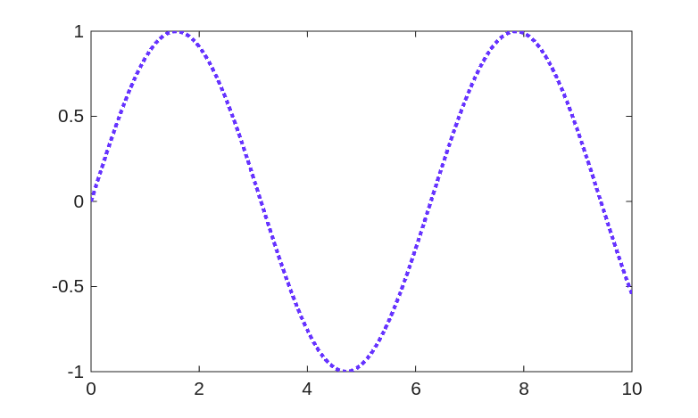
../_images/tutorial-1-plot-1.png — The generated plot using the style defined in `config.yaml`.¶

Finally, open config.yaml in the MATLAB editor and manually change LineWidth: 2.0 to LineWidth: 5.0. Save the file, then run the previous commands again. Notice that style of the plot has changed without modifying the MATLAB code itself.

Optional challenges¶

Let’s take it a step further with these optional challenges.

Challenge 1: Create a library of YAML files¶

The task of this challenge is to create a library of YAML files with different style configurations. For example, you could create green.yaml and dashed.yaml as follows:

green.yaml¶

LineStyle: '-'
LineWidth: 1.5
Color: [0.3, 0.76, 0.4]

dashed.yaml¶

LineStyle: '--'
LineWidth: 1
Color: [0.0, 0.0, 0.0]

And then, to switch between styles, you only need to change which YAML file you are loading:

>> x = 0:0.1:10;
>> y1 = sin(x);
>> y2 = cos(x);
>> figure;
>> hold on;
>> plot_yaml(x, y1, 'green.yaml');
>> plot_yaml(x, y2, 'dashed.yaml');

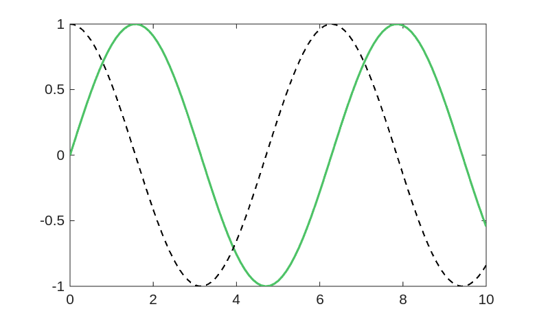
../_images/tutorial-1-plot-2.png — The generated plot using the style defined in `green.yaml` and `dashed.yaml`.¶

Challenge 2: Add more style options¶

The task of this challenge is to add more style options (for example, line marker types, axis limits, titles or labels) by including more information in the YAML files and updating the plot_yaml() function accordingly.

Here is an example of how you could add an option to specify whether the gird is on or off:

config.yaml (updated)¶

LineStyle: ':'
LineWidth: 2
Color: [0.4, 0.2, 1.0]
Grid: 'on'

plot_yaml.m (updated)¶

function plot_yaml(x, y, config_file)
%PLOT_YAML Plot data using style options defined in a YAML file
%
%   PLOT_YAML(x, y, config_file) plots y versus x using line style
%   parameters loaded from the YAML configuration file specified by
%   configFile.

    % Load the configuration of the YAML file.
    config = yaml.loadFile(config_file, 'ConvertToArray', true);

    % Plot using the style configuration.
    plot(x, y, ...
        'LineStyle', config.LineStyle, ...
        'LineWidth', config.LineWidth, ...
        'Color', config.Color);

    % Set the grid style.
    grid(config.Grid);
end

>> x = 0:0.1:10;
>> y = sin(x);
>> plot_yaml(x, y, 'config.yaml');

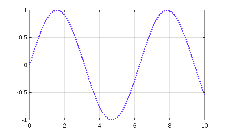
../_images/tutorial-1-plot-3.png — The generated plot using the updated `config.yaml` and `plot_yaml()` function.¶

Wrap-Up: What you’ve learned and next steps¶

Congratulations! You have succesfully used YAML in MATLAB. By using yaml.dumpFile() and yaml.loadFile(), you built a workflow where the configuration style of plots is separated from the MATLAB code. This is a best practice that makes your code more flexible, readable, and reproducible.

While styling plot() is a simple starting point, this configuration-driven approach is powerful. You can apply these same principles to manage simulation parameters, hardware settings, or complex model analysis without ever hard-coding values into your scripts.

Ready to go further?¶

To continue your journey with YAML and MATLAB, consider these next steps:

Explore YAML syntax. Explore the YAML syntax for defining the different data types and nested structures and learn how to write YAML files manually
Explore YAML package. Check the API Reference to learn about the rest of the available functions and their options.